
Positional Encodings and Extension Methods
Published:
Abstract
This post reviews common positional encoding methods and approaches to extending the context length of language models, from sinusoidal embeddings and relative position biases to RoPE and its extensions. Alongside their mathematical formulations, I share my understanding of how these methods encode position, interact with token content, and behave beyond the training context length—why they work, where they fail, and what their limitations reveal. The aim is to connect the intuition behind positional encodings with the design choices and trade-offs of context extension.
1. Position Encodings
1.1 Sinusoidal position encoding
Notation
| Symbol | Meaning |
|---|---|
| \(pos\) | Token position (starting from 0). |
| \(d\) | Model/embedding dimension; assumed even here. |
| \(i\) | Dimension-pair index, 0 to d/2−1; not a token position in this section. |
| \(\mathrm{PE}(pos,2i),\mathrm{PE}(pos,2i+1)\) | Sine and cosine components of the positional encoding. |
| \(k\) | Fixed offset between token positions. |
| \(\pi\) | The circle constant; one complete rotation is 2π radians. |
The original Transformer1 adds a fixed encoding to the token embedding at each position \(pos\). For \(i = 0, \dots, d/2-1\), where \(d\) is the model dimension,
\[ \mathrm{PE}(pos, 2i) = \sin\left(\frac{pos}{10000^{2i/d}}\right), \qquad \mathrm{PE}(pos, 2i + 1) = \cos\left(\frac{pos}{10000^{2i/d}}\right). \]
- The periods range from \(2\pi\) (fastest band) to about \(20000\pi\) (slowest band).
- The authors hypothesized that this lets the model easily learn to attend by relative positions, because \(\mathrm{PE}(pos + k)\) is a linear function of \(\mathrm{PE}(pos)\) for any fixed offset \(k\).
1.2 Learnable absolute position encoding
Each position has its own learnable embedding, which is added to the token embedding at that position. The positional embeddings are randomly initialized and trained together with the model.
- Applied by BERT2 and GPT3
- Described as an improvement upon the sinusoidal position encoding4
- The number of positions is fixed at training time, so the model cannot take longer inputs at all
1.3 T5 relative bias5
Notation
| Symbol | Meaning |
|---|---|
| \(i,j\) | Query and key token positions (a different use of i from §1.1). |
| \(l,h\) | Layer index and attention-head index. |
| \(q_i^{(l,h)},k_j^{(l,h)}\) | Query and key vectors at the indicated layer and head. |
| \(s(i,j)^{(l,h)}\) | Attention logit before softmax. |
| \(M_{i,j}\) | Attention-mask bias: typically 0 for allowed pairs and −∞ for blocked pairs. |
| \(d\) | Relative distance |i−j| in the bucket formula; not the embedding dimension here. |
| \(B,D\) | Number of buckets and maximum-distance parameter (far distances share the last bucket). |
| \(g(d),\mathrm{bucket}(d)\) | Bucket index assigned to distance d; logarithmic indices are rounded down. |
| \(b^{(h)}\) | Learned positional-bias table for head h, shared across layers. |
| \(\top,\log,\min\) | Transpose, logarithm, and minimum. |
T5 doesn’t add positional embeddings to individual positions, but directly adds a bias to each logit. The bias is determined by the relative position.
For position \(i\) and \(j\) at layer \(l\) and head \(h\), the logit \(s_{i, j}^{(h, l)}\) is defined as
\[ s(i, j)^{(l,h)} = (q_i^{(l,h)})^\top k_j^{(l,h)} + b_{\textrm{bucket}(\mid i-j\mid)}^{(h)} + M_{i,j}, \]
where \(b_{\textrm{bucket}(d)}^{(h)}\) is the positional bias of relative distance \(d\) at head \(h\). In the T5 implementation, the positional biases are shared between layers so there is only \(h\) index at its superscript.
The bucket is designed to give fine resolution to recent positions and coarse resolution to far positions. Assume the number of buckets is \(B\), max distance is \(D\), the bucket index \(g(d)\) is defined as
\[ g(d) = \begin{cases} d & d < B/2 \\ \min(B - 1, B/2 + \frac{\log(2d/B)}{\log(2D/B)}\cdot\frac{B}{2}) & d \geq B/2. \end{cases} \]
In this case, each closest relative position gets one bucket, the farther the larger the bucket (coarser resolution).
For example, with a toy setting \(B = 8\) and \(D = 64\) (bucket index rounded down; T5 itself uses \(B = 32\), \(D = 128\)):
| \(d\) | 0 | 1 | 2 | 3 | 4–7 | 8–15 | 16–31 | ≥32 |
|---|---|---|---|---|---|---|---|---|
| bucket | 0 | 1 | 2 | 3 | 4 | 5 | 6 | 7 |
1.3.1 T5 relative bias is a biased NoPE
Notation
| Symbol | Meaning |
|---|---|
| \(q_i,k_j\) | Content query/key vectors; layer and head indices are omitted. |
| \(p_i^q,p_j^k\) | Additive positional vectors for the query and key; q/k superscripts are labels. |
| \(i-j\) | Signed relative position. |
💡 My thinking about relative bias
For additive position encodings \(p\), adding them to \(q\) and \(k\) is equivalent to adding biases to the logits:
\[ (q_i + p^q_i)^\top (k_j + p^k_j) = (q_i)^\top k_j + (q_i)^\top p_j^k + (p_i^q)^\top k_j + (p_i^q)^\top p_j^k \]
Here \((p_i^q)^\top p_j^k\) is a bias that depends only on the positions, while \((q_i)^\top p_j^k + (p_i^q)^\top k_j\) is a bias determined by the interaction between semantics and positions.
However, these biases generally depend on the absolute positions \(i\) and \(j\), which is undesirable. We want the positional effect to depend only on the relative distance \(i - j\).
The T5 relative bias depends only on the relative distance, but it has no interaction between semantics and positions. Such an interaction is still useful. For example, the meaning of the token “tion” relies heavily on the previous token, while the token “France” relies much less on it. How much a token attends to its neighbors therefore depends on its semantics. We need positional biases that depend on both the semantics and the relative distance, but not on the absolute positions. This is what RoPE 6 provides.
But why does the T5 relative bias still work without this semantic dependency? One reason is that the model can build it across layers: a head with a strong local bias can copy the previous token into the current hidden state, so later layers already see position-aware content in \(q\) and \(k\). In a causal decoder, the causal mask also leaks order information, since a token can infer its position from how many tokens it can see. This is why causal language models without any positional encoding (NoPE) still learn positional information7.
So basically, the T5 relative bias is NoPE plus a learned, per-head bias on the bucketed relative distance. This bias is not constrained to decay with distance, and all distances beyond \(D\) share the last bucket
1.4 Rotary position embedding (RoPE)
Notation
| Symbol | Meaning |
|---|---|
| \(q_i,k_j\) | Query at position i and key at position j. |
| \(f(x,m)\) | Position-dependent transformation of vector x at position m. |
| \(g(q_i,k_j,i-j)\) | Desired content-and-relative-position function; unrelated to T5’s bucket g. |
| \(s_{\mathrm{RoPE}}(i,j)\) | RoPE attention logit. |
As shown above, additive position encodings generally make the logits depend on the absolute positions, while the T5 relative bias lacks the semantic-position interaction. Su et al. 6 later proposed RoPE, which keeps this interaction but makes it depend only on the relative position, while being more expressive than bucketed biases.
The target of RoPE is to encode positions such that the logit \(s(i,j)\) is a function of the contents and the relative distance only
\[ s_{\textrm{RoPE}}(i,j) = f(q_i, i)^{\top} f(k_j, j) = g(q_i, k_j, i-j) \]
1.4.1 Intuition behind RoPE
Notation
| Symbol | Meaning |
|---|---|
| \(z,z_1,z_2\) | Complex numbers. |
| \(c,c_1,c_2\) | Complex-number magnitudes (lengths). |
| \(\theta,\theta_1,\theta_2\) | Complex-number angles, in radians. |
| \(\mathrm{i}\) | Imaginary unit, √−1; distinct from the position index i. |
| \(\bar z,\exp\) | Complex conjugate and exponential function. |
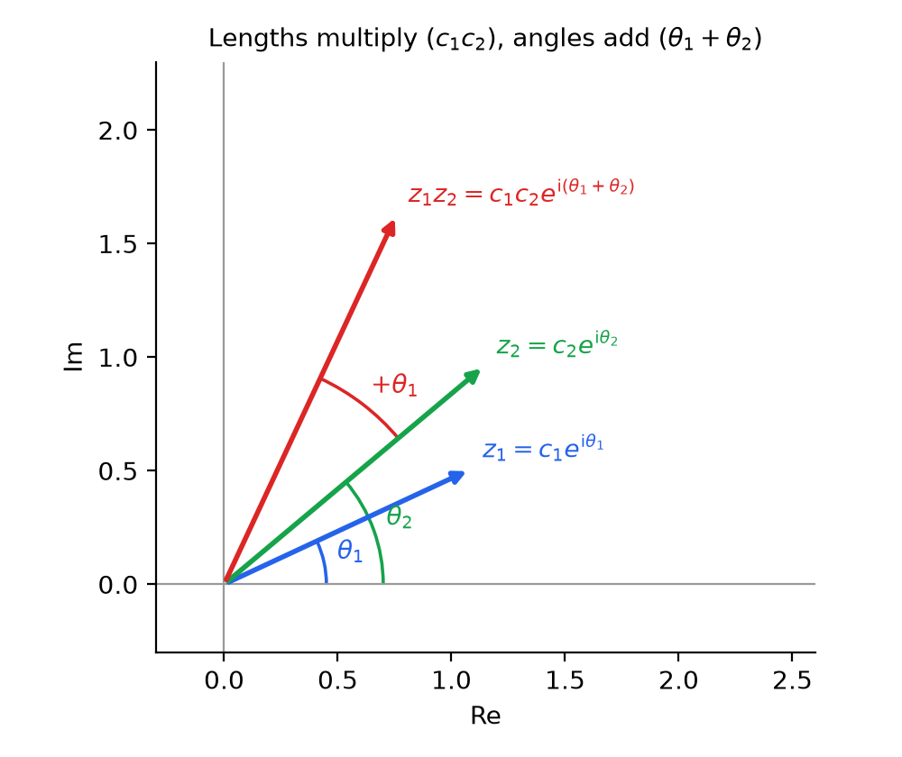
Any complex number can be expressed by a modulus (length) \(c\) and an angle \(\theta\) from the positive real axis
\[ z = c\exp(\mathrm{i}\theta) \]
Multiplying two complex numbers simply multiplies the moduli and adds the angles.
\[ z_1 \times z_2 = c_1 c_2 \exp(\mathrm{i}(\theta_1 + \theta_2)) \]
If we multiply the first complex number by the conjugate of the second, the result only depends on the moduli and their relative angle.
\[ z_1 \times \bar{z}_2 = c_1 c_2 \exp(\mathrm{i}(\theta_1 - \theta_2)) \]
The relative angle \(\theta_1 - \theta_2\) is what we can use to express the relative distance!
1.4.2 RoPE
Notation
| Symbol | Meaning |
|---|---|
| \(d,t\) | Even head dimension and dimension-pair index t=0,…,d/2−1. |
| \(q_{i,2t},q_{i,2t+1}\) | Two real components forming pair t of the query at position i. |
| \(\tilde q_i^{(t)},\tilde k_j^{(t)}\) | Complex representation of query/key pair t. |
| \(\theta_t\) | Angular frequency of pair t; smaller t denotes faster rotation. |
| \(\mathbb R^d,\mathrm{Re},\sum\) | d-dimensional real vector space, real part, and summation over pairs. |
For simplicity, we introduce RoPE with a single-head attention and ignore the attention mask (causal mask).
Let \(q_i, k_j \in \mathbb{R}^{d}\) (\(d\) even) be the query at position \(i\) and the key at position \(j\). Split the dimensions into \(d/2\) pairs \((2t, 2t+1)\) and view each pair as a complex number \(\tilde{q}_i^{(t)} = q_{i,2t} + \mathrm{i}\, q_{i,2t+1}\) (same for \(\tilde{k}_j^{(t)}\)), with frequency \(\theta_t = 10000^{-2t/d}\), \(t = 0, \dots, d/2-1\).
Transformation. Rotate pair \(t\) by the angle (position \(\times\, \theta_t\)):
\[ f(q_i, i)^{(t)} = \tilde{q}_i^{(t)} \exp(\mathrm{i}\, i\theta_t), \qquad f(k_j, j)^{(t)} = \tilde{k}_j^{(t)} \exp(\mathrm{i}\, j\theta_t). \]
Logits.
\[ s_{\textrm{RoPE}}(i,j) = \mathrm{Re}\left[ \sum_{t=0}^{d/2-1} f(q_i, i)^{(t)}\, \overline{f(k_j, j)^{(t)}} \right] = \mathrm{Re}\left[ \sum_{t=0}^{d/2-1} \tilde{q}_i^{(t)}\, \overline{\tilde{k}_j^{(t)}}\, \exp(\mathrm{i}(i-j)\theta_t) \right], \]
which depends on the positions only through \(i - j\).
1.4.3 Implementation of RoPE
Notation
| Symbol | Meaning |
|---|---|
| \(a_1,b_1,a_2,b_2\) | Real and imaginary components of z₁ and z₂. |
| \(q_a,q_b,k_a,k_b\) | Real and imaginary halves of the query and key vectors. |
| \(m,\theta\) | Token position and vector of per-pair frequencies. |
| \(u_m,v_m\) | Element-wise cos(mθ) and sin(mθ). |
| \(\odot,[q_a;q_b]\) | Element-wise multiplication and concatenation of the two halves. |
| \(e\) | Base of the natural logarithm; exp(x)=eˣ. |
The product of two complex numbers could be expressed as
\[ \begin{align} z_1 \times \overline{z_2} &= (a_1 + \mathrm{i}b_1) \times \overline{(a_2 + \mathrm{i}b_2)} \\ &= (a_1 + \mathrm{i}b_1) \times (a_2 - \mathrm{i}b_2)\\ &= a_1a_2 + b_1b_2 + \mathrm{i}(a_2b_1 - a_1b_2). \end{align} \]
Thus, the real part is simply
\[ \textrm{Re} \left[z_1 \times \overline{z_2} \right] = a_1a_2 + b_1b_2, \]
which is just the real dot product of \((a_1, b_1)\) and \((a_2, b_2)\). So we never need complex numbers: rotate \(q\) and \(k\) as real vectors, then take the ordinary dot product.
Split into halves. Store a complex vector as its real half and imaginary half: \(q = [q_a; q_b]\) means \(\tilde{q} = q_a + \mathrm{i}\, q_b\) (same for \(k\)). Then
\[ \mathrm{Re}\left[\sum \tilde{q} \odot \overline{\tilde{k}}\right] = q_a^\top k_a + q_b^\top k_b = q^\top k, \]
so the logit is just the ordinary dot product of the two real vectors.
Rotation. Rotating \(\tilde{q}\) at position \(m\) means multiplying by \(e^{\mathrm{i} m\theta} = u_m + \mathrm{i}\, v_m\), where \(u_m = \cos(m\theta)\) and \(v_m = \sin(m\theta)\) are vectors (one entry per frequency). With the halves this is only element-wise multiplications and additions:
\[ \mathrm{RoPE}(q, m) = \begin{bmatrix} q_a \odot u_m - q_b \odot v_m \\ q_a \odot v_m + q_b \odot u_m \end{bmatrix} = q \odot \begin{bmatrix} u_m \\ u_m \end{bmatrix} + \begin{bmatrix} -q_b \\ q_a \end{bmatrix} \odot \begin{bmatrix} v_m \\ v_m \end{bmatrix}, \]
and the same for \(k\) at its own position. The logit is \(\mathrm{RoPE}(q, i)^\top \mathrm{RoPE}(k, j)\).
What is precomputed. The frequencies \(\theta\) are fixed, so \(u_m\) and \(v_m\) for every position \(m\) up to the maximum length are computed once and stored as a cos table and a sin table. At run time we only look up the rows for the current positions and do the element-wise operations above. During generation, the KV cache stores the keys after rotation, so each key is rotated only once (this assumes the rotation of a token never changes; see 2.3.1 for the case where it does).
1.4.4 Influence
RoPE is the de-facto position encoding method in recent open-source LLM literature.
- LLaMA series
- Qwen series
- Gemma series
- Mistral series
- DeepSeek series
- …
1.4.5 Why RoPE succeeded
This section is based on my own understanding.
💡 In the original paper, the authors state: “Notably, RoPE enables valuable properties, including the flexibility of sequence length, decaying inter-token dependency with increasing relative distances, and the capability of equipping linear self-attention with relative position encoding”. However, I think the long-term decay is not what the model actually relies on.
The paper only proves that an upper bound of the logit decays with distance, and Barbero et al. 8 show that this decay does not hold in general (e.g. for random queries and keys). The distance preference that trained models actually show comes mainly from the functional split between attention heads, not from RoPE’s decay.
In my understanding, RoPE succeeds because it provides a positional bias that depends on both the semantics and the relative distance, but not on the absolute positions (see 1.3).
1.5 XPos
Notation
| Symbol | Meaning |
|---|---|
| \(i,j,t,d\) | Query/key positions, pair index, and even head dimension, as in RoPE. |
| \(\zeta_t\) | Per-pair decay rate between 0 and 1. |
| \(\lambda\) | Decay-shape parameter, set to 0.4; not the wavelength λₜ used later. |
| \(\gamma\) | Distance scale for decay, set to 512; not YaRN’s blending coefficient γₜ. |
| \(s_{\mathrm{XPos}}(i,j)\) | Attention logit after rotary encoding and decay. |
Previously, people thought that models cannot work beyond the training length because of the absolute position encoding. However, RoPE-based models, although they remove the dependence on absolute positions, still cannot work beyond the training length.
Sun et al. 9attribute this to the fast-rotating bands: at large distances they make the logits oscillate instead of decaying, which adds noise to attention and hinders the extrapolation of RoPE. Thus, they add an explicit distance decay to RoPE. Each dimension pair \(t = 0, \dots, d/2-1\) (the same pair index as in 1.4.2, so small \(t\) means a fast band) gets a decay rate
\[ \zeta_t = \frac{2t/d + \lambda}{1 + \lambda} \in (0, 1), \qquad \lambda = 0.4, \]
and the query and key are scaled in opposite directions before rotation:
\[ f(q_i, i)^{(t)} = \tilde{q}_i^{(t)}\, \zeta_t^{\,i/\gamma} \exp(\mathrm{i}\, i\theta_t), \qquad f(k_j, j)^{(t)} = \tilde{k}_j^{(t)}\, \zeta_t^{-j/\gamma} \exp(\mathrm{i}\, j\theta_t), \]
with \(\gamma = 512\). The logit becomes
\[ s_{\textrm{XPos}}(i,j) = \mathrm{Re}\left[ \sum_{t} \tilde{q}_i^{(t)}\, \overline{\tilde{k}_j^{(t)}}\, \zeta_t^{(i-j)/\gamma} \exp(\mathrm{i}(i-j)\theta_t) \right], \]
which still depends only on \(i - j\), and for \(i \ge j\) (causal attention) each band is damped by \(\zeta_t^{(i-j)/\gamma}\). Fast bands (small \(t\), small \(\zeta_t\)) decay quickly, so they only matter for nearby tokens; slow bands (\(\zeta_t \to 1\)) barely decay. At inference, XPos is also combined with blockwise causal attention to extrapolate to longer sequences.
However, the experiments are small: a model comparable to GPT-3 Medium (24 layers, 1024 hidden) is trained from scratch with length 1024 and evaluated on arXiv only up to 4096, i.e. 4× the training length. With blockwise causal attention, the perplexity keeps dropping (23.31 → 21.6 → 20.73 at 1024 / 2048 / 4096), but plain RoPE with blockwise causal attention also stops exploding (25.57 / 25.65 vs. 73.6 / 294.45 without it). Without it, XPos still degrades (22.56 at 2048, 28.43 at 4096), so the decay alone does not solve extrapolation, and much of the gain comes from the windowed attention.
Decay the fast bands may help far tokens, but it’s better to preserve the fast bands in recent tokens.
1.6 Attention with linear biases (ALiBi)
Notation
| Symbol | Meaning |
|---|---|
| \(s_{\mathrm{ALiBi}}(i,j)\) | Attention logit with a linear distance penalty. |
| \(H,h\) | Number of heads and head index h=1,…,H. |
| \(m_h\) | Positive distance-penalty slope for head h; the stated geometric formula is the power-of-two-head case. |
| \(i-j,\exp(x)\) | Nonnegative causal distance and exponential weighting induced by softmax. |
Similar to XPos (though published earlier), Press et al. 10 proposed ALiBi to decay the attention scores of far tokens. ALiBi adds no position embedding to \(q\) or \(k\); instead it adds a fixed, non-learned linear penalty to each logit:
\[ s_{\textrm{ALiBi}}(i,j) = q_i^\top k_j - m_h\,(i-j), \qquad j \le i, \]
where \(m_h\) is a head-specific slope. For \(H\) heads the slopes form a geometric sequence \(m_h = 2^{-8h/H}\), \(h = 1, \dots, H\) (e.g. \(\frac{1}{2}, \frac{1}{4}, \dots, \frac{1}{256}\) for 8 heads).
Unlike XPos, which multiplies the logits by a decay factor (pushing far logits towards \(0\)), ALiBi adds a penalty that goes to \(-\infty\) with distance, so far tokens are truly suppressed after softmax. Each head therefore works as a soft sliding window of a different size: with \(m_h = 1/2\), a token 20 positions away is already down-weighted by \(e^{-10}\), while with \(m_h = 1/256\) the penalty at distance 2048 is only \(-8\). A 1.3B model trained on length 1024 extrapolates to 2048 with the same perplexity as a sinusoidal model trained on 2048, and the perplexity stays stable at much longer lengths. ALiBi was later used by BLOOM and MPT.
1.6.1 ALiBi is a NoPE with distance decay
The positional bias \(-m_h\,(i-j)\) depends only on the relative distance, not on the semantics. Like the T5 relative bias, ALiBi is therefore NoPE plus a relative bias, but here the bias is fixed and always decays with distance. Since the decay is strong in most heads, far tokens are largely ignored and the model behaves like a streaming LLM. Thus, ALiBi is functionally similar to a streaming NoPE, except that the heads with the smallest slopes can still see far tokens.
2. Training-free Context Extension
Notation
| Symbol | Meaning |
|---|---|
| \(L,L'\) | Training context length and target extended context length. |
| \(s\) | Extension factor L′/L>1; not the attention logit s(i,j). |
| \(i,j,t,\theta_t\) | Query/key positions, frequency-band index, and original angular frequency. |
A RoPE model trained with context length \(L\) fails on longer inputs mainly because the angle \((i-j)\theta_t\) in the logit
\[ s_{\textrm{RoPE}}(i,j) = \mathrm{Re}\left[ \sum_{t} \tilde{q}_i^{(t)}\, \overline{\tilde{k}_j^{(t)}}\, \exp(\mathrm{i}(i-j)\theta_t) \right] \]
leaves the range seen during training. To use the model at length \(L' = sL\) (\(s > 1\)) without changing its architecture, we can change the frequencies \(\theta_t\) (2.1) or the distance \(i - j\) (2.2). Either can also follow the current sequence length instead of being fixed up front (2.3).
2.1 Rescaling the frequencies
Notation
| Symbol | Meaning |
|---|---|
| \(\theta_t,\theta'_t\) | Original and rescaled angular frequencies of band t. |
These methods slow down the rotation speed \(\theta_t\) to \(\theta'_t\). They differ in how much each band is scaled.
2.1.1 Position Interpolation (PI)
Notation
| Symbol | Meaning |
|---|---|
| \(s,m\) | Extension factor and token position before interpolation. |
| \(m/s\) | Interpolated (possibly fractional) token position. |
Chen et al. 11 and, concurrently, kaiokendev 12 scale all bands equally:
\[ \theta'_t = \frac{\theta_t}{s}. \]
Position \(m\) now has the angles of position \(m/s\), so all positions up to \(L'\) stay in the seen range. However, nearby tokens now differ by only \(1/s\) of a position, so the fast bands lose resolution and PI relies on fine-tuning to recover it. With fine-tuning within 1000 steps, LLaMA is extended to 32768.
2.1.2 NTK-aware scaling
Notation
| Symbol | Meaning |
|---|---|
| \(t,d\) | Pair index and even head dimension (d>2 for this formula). |
| \(s^{-2t/(d-2)}\) | Frequency-scaling factor for pair t. |
To keep the fast bands, bloc97 13 scale the bands non-uniformly, motivated by the NTK analysis of Fourier features 14: high-frequency inputs are needed to learn high-frequency functions. This is done by enlarging the base in \(\theta_t\), which is equivalent to
\[ \theta'_t = \theta_t \cdot s^{-2t/(d-2)}. \]
The fastest band is unchanged and only the slowest band is scaled by the full \(1/s\). This works much better than PI without fine-tuning. However, the other bands are scaled by less than \(1/s\), so some of them still reach out-of-bound angles: Peng et al. 4 report that it is inferior to PI after fine-tuning, and that \(s\) must be set higher than the expected extension.
2.1.3 YaRN
Notation
| Symbol | Meaning |
|---|---|
| \(\lambda_t\) | Wavelength of band t, 2π/θₜ, measured in token positions. |
| \(r_t\) | Number of rotations within the training length: L/λₜ. |
| \(\alpha,\beta\) | Lower/upper rotation-count thresholds; 1 and 32 in the stated Llama setting. |
| \(\gamma_t\) | Blending weight from 0 (full interpolation) to 1 (unchanged frequency). |
| \(\tau\) | Attention temperature; q and k are each multiplied by √(1/τ). |
| \(d,\ln,\mathrm{softmax}\) | Head dimension, natural logarithm, and normalization of logits into attention weights. |
Peng et al. 4 scale each band according to how many turns it makes during the training context length, \(r_t = L / \lambda_t\), where \(\lambda_t = 2\pi / \theta_t\) is its wavelength. This NTK-by-parts interpolation 15 is
\[ \theta'_t = (1 - \gamma_t)\, \frac{\theta_t}{s} + \gamma_t\, \theta_t, \qquad \gamma_t = \min\left(1, \max\left(0, \frac{r_t - \alpha}{\beta - \alpha}\right)\right), \]
with \(\alpha = 1\), \(\beta = 32\) for Llama. Fast bands (\(r_t > \beta\)) have seen every angle, so they stay unchanged. Slow bands (\(r_t < \alpha\)) never finish one turn, so they are scaled by the full \(1/s\) as in PI. Bands in between are blended.
💡 My understanding
Both methods scale the rotation speed of each band by a factor between \(1\) (unchanged) and \(1/s\) (as in PI). NTK-aware scaling spreads this factor over all bands geometrically in the band index \(t\): \(s^{-2t/(d-2)}\) goes from \(1\) at the fastest band to \(1/s\) only at the slowest one. YaRN instead interpolates linearly in the number of turns \(r_t\) (i.e. in the frequency, not the band index), and \(\alpha\) and \(\beta\) set the blending range in turns: bands with \(r_t > \beta\) keep factor \(1\), bands with \(r_t < \alpha\) get the full \(1/s\).
As a longer context also flattens the attention, YaRN sharpens it with a temperature \(\tau\), applied by scaling both \(q\) and \(k\) by \(\sqrt{1/\tau}\):
\[ \mathrm{softmax}\left(\frac{q_i^\top k_j}{\tau\sqrt{d}}\right), \qquad \sqrt{1/\tau} = 0.1 \ln s + 1 . \]
Llama 2 7B / 13B (trained on 4096) reach 64k (\(s = 16\)) with 400 fine-tuning steps and 128k (\(s = 32\)) with 200 more, using about 0.1% of the pre-training data.
2.2 Remapping the relative distance
Notation
| Symbol | Meaning |
|---|---|
| \(\delta(i,j)\) | Remapped relative distance between query i and key j. |
| \(s_\delta(i,j)\) | Attention logit using the remapped distance; original frequencies are retained. |
These methods keep \(\theta_t\) and replace \(i - j\) with a mapped distance \(\delta(i, j)\):
\[ s_{\delta}(i,j) = \mathrm{Re}\left[ \sum_{t} \tilde{q}_i^{(t)}\, \overline{\tilde{k}_j^{(t)}}\, \exp(\mathrm{i}\, \delta(i,j)\, \theta_t) \right], \qquad j \le i. \]
They all keep the exact distance for nearby tokens, which language modeling depends on, and give far tokens a coarser distance. They differ in how coarse it is.
2.2.1 ReRoPE
Notation
| Symbol | Meaning |
|---|---|
| \(w\) | Local-window distance threshold, smaller than training length L. |
| \(\min(i-j,w)\) | Exact local distance, capped at w for remote tokens. |
Rectified RoPE 16 is the coarsest case. It caps the distance at a window \(w < L\), so all tokens beyond \(w\) look equally far:
\[ \delta(i,j) = \min(i - j, w). \]
On Llama 2 13B with \(w = 1024\), the loss is 1.50 / 1.43 / 1.40 at 4k / 8k / 16k, while plain RoPE jumps from 1.50 at 4k to 8.86 at 8k. Its implementation needs two attention passes and, at the time of An et al. 17, was not compatible with FlashAttention.
This is an engineering limitation rather than an algorithmic one. ReRoPE needs two logits per query-key pair, the usual RoPE one and one with the fixed distance \(w\), and picks one of them before the softmax. The stock FlashAttention kernel does not expose the logits, so this needs a custom kernel or a merge of several standard attention calls. Jet-Long (2.3.2) does exactly this for a similar local / remote split and keeps 83–88% of the FlashAttention-3 prefill throughput.
2.2.2 Self-Extend
Notation
| Symbol | Meaning |
|---|---|
| \(G,w\) | Group size and local-window distance threshold. |
| \(\lfloor x\rfloor\) | Floor: largest integer no greater than x. |
| \(\lfloor i/G\rfloor,\lfloor j/G\rfloor\) | Query/key group indices. |
| \(L,L'\) | Training context length and desired extended length. |
Instead of one distance for all far tokens, Jin et al. 18 group them: with a neighbor window \(w\) and a group size \(G\), the tokens of a group share the position \(\lfloor i / G \rfloor\):
\[ \delta(i,j) = \begin{cases} i - j & i - j \le w \\ \lfloor i / G \rfloor - \lfloor j / G \rfloor + w - \lfloor w / G \rfloor & \text{otherwise.} \end{cases} \]
The shift \(w - \lfloor w / G \rfloor\) joins the two parts smoothly, and the context is extended up to \((L - w)G + w\). ReRoPE is the special case where \(G\) is so large that all far tokens fall into one group.
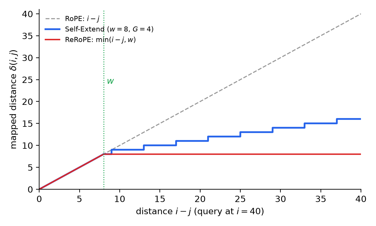
For a query at position \(i\), nearby tokens keep their exact distance, while far tokens are grouped \(G\) at a time onto the same position, so the distance becomes a staircase (figure above, \(w = 8\), \(G = 4\)).
\(G\) is chosen in advance from the target length \(L'\): to cover \(L'\) we need \((L - w)G + w \ge L'\), i.e. \(G \ge (L' - w)/(L - w)\). For example, Llama 2 with \(L = 4096\) and \(w = 1024\) needs \(G \ge 5\) for 16k. Since \(G\) is fixed and groups are defined by absolute positions \(\lfloor j/G \rfloor\), the group of a cached key never changes as the sequence grows, so its grouped rotation can be cached as well. The cost is two sets of logits (neighbor and grouped) merged before the softmax.
Without fine-tuning, the perplexity of Llama-2-7B-chat on PG-19 stays around 9 up to 12288, while the original model exceeds \(10^3\) from 6144. Mistral 7B reaches 100% on passkey retrieval, whereas a sliding window has low perplexity but cannot retrieve anything outside the window, so low perplexity alone does not prove long-context ability.
2.2.3 Dual Chunk Attention (DCA)
Notation
| Symbol | Meaning |
|---|---|
| \(c\) | Chunk size, smaller than L; not the complex magnitude c from §1.4.1. |
| \(a,b\) | Query/key positions within their chunks: i mod c and j mod c. |
| \(\lfloor i/c\rfloor,\lfloor j/c\rfloor\) | Query/key chunk indices. |
| \(\bmod,L\) | Remainder operation and training context length. |
An et al. 17 split the sequence into chunks of size \(c < L\). With \(a = i \bmod c\) and \(b = j \bmod c\) the positions inside each chunk,
\[ \delta(i,j) = \begin{cases} a - b & \lfloor i/c \rfloor - \lfloor j/c \rfloor = 0 \quad \text{(intra-chunk)} \\ \min(c + a, L - 1) - b & \lfloor i/c \rfloor - \lfloor j/c \rfloor = 1 \quad \text{(successive-chunk)} \\ L - 1 - b & \lfloor i/c \rfloor - \lfloor j/c \rfloor > 1 \quad \text{(inter-chunk)} \end{cases} \]
Intra-chunk attention keeps the exact distance. Successive-chunk attention also keeps it for the first \(L - c\) positions of a chunk, so tokens right after a boundary do not lose their neighbors. Inter-chunk attention gives every query the largest position \(L - 1\), so far keys only keep their order inside a chunk.
Since \(a \le c - 1\), the cap \(\min(c + a, L - 1)\) only takes effect when \(2c > L\). Otherwise the whole previous chunk is within distance \(L - 1\) and successive-chunk attention is exact for every key. The example in An et al. 17 uses \(c = 6\) with \(L = 10\), i.e. \(c > L/2\).
In implementation, each key is rotated once at its in-chunk position \(b\) and cached. Each query is rotated to three positions, \(a\), \(\min(c + a, L - 1)\) and \(L - 1\), and uses the one that matches the chunk of the key. The three cases cover disjoint sets of keys (same chunk, previous chunk, earlier chunks), so attention is computed as three standard FlashAttention calls merged by their log-sum-exp statistics, with the same total cost as full attention.
DCA can be applied on top of PI or NTK-aware models. Without fine-tuning, it extends Llama 2 70B from 4k to 96k with a perplexity increase of 0.56.
2.2.4 Dimension-Wise Positional Embeddings Manipulation (DPE)
Notation
| Symbol | Meaning |
|---|---|
| \(g,e_g\) | Frequency-group index and measured effective length of group g. |
| \(l\) | Current sequence length; not the layer index l in §1.3. |
| \(\sigma_g\) | Distance-compression factor ⌊l/e_g⌋ for group g, in the extension regime where it is positive. |
| \(\delta_t(i,j)\) | Remapped distance specifically for band t. |
| \(\lVert q^{(t)}\rVert\lVert k^{(t)}\rVert\) | Product of query/key pair norms, used as a contribution measure (position indices omitted). |
| \(w,t,d\) | Local-window threshold, pair index, and even head dimension. |
The methods above apply the same \(\delta\) to all bands. Lu et al. 19 remap each band separately, based on two findings on Llama 3 8B:
- Bands have different effective lengths: the fastest and the slowest bands still work when the distance exceeds the training range, while the middle bands fail immediately.
- Only some bands matter: most of the contribution \(\lVert q^{(t)} \rVert \lVert k^{(t)} \rVert\) comes from a few bands, which differ across heads and layers.
DPE therefore splits the bands into 8 groups and measures the effective length \(e_g\) of each group with a retrieval task. For each head, it selects the top-48 bands by the contribution above and remaps only these bands, leaving the others at \(i - j\). For a selected band \(t\) in group \(g\), with a local window \(w = 1\)k,
\[ \delta_t(i,j) = \begin{cases} \lfloor (i - j - w) / \sigma_g \rfloor + w & i - j > w \\ i - j & \text{otherwise,} \end{cases} \qquad \sigma_g = \lfloor l / e_g \rfloor , \]
where \(l\) is the sequence length. Without fine-tuning, DPE extends Llama 3 8B from 8k to 128k with a Needle-in-a-Haystack accuracy of 92.5% (Self-Extend: 89.5%, ReRoPE: 78%, DCA: 53%, YaRN: 0%).
Unlike YaRN, which fully interpolates the slowest bands, DPE finds that they tolerate longer distances. A possible explanation (not from the paper): with Llama 3’s base \(500000\) (instead of \(10000\)), the slowest bands (the last group, \(t \ge 56\)) rotate less than a quarter turn even at 128k, while the middle bands make at most a few turns within 8k but many more at 128k.
2.3 Following the current length
Notation
| Symbol | Meaning |
|---|---|
| \(l,L,s,G\) | Current length, training length, frequency-extension factor, and distance-group size. |
The methods above fix \(s\) or \(G\) up front, which is a trade-off: a large value hurts short inputs, and a small value breaks on long inputs. Instead, the setting can follow the current sequence length \(l\), so that the model stays unchanged for \(l \le L\).
2.3.1 Dynamic scaling
Notation
| Symbol | Meaning |
|---|---|
| \(s=\max(1,l/L)\) | Length-dependent extension factor; equals 1 within the training length. |
Frequency methods can update \(s\) at every forward pass, so performance degrades gracefully instead of abruptly beyond \(L'\):
\[ s = \max(1, l / L). \]
Combined with NTK-aware scaling this is Dynamic NTK 20. Dynamic-YaRN gives more than 2× extension without any fine-tuning. As the rotation of every token changes with \(s\), the KV cache must store the keys before applying RoPE.
💡 Dynamic NTK and Dynamic-YaRN are just dynamic versions of NTK and YaRN. They need to rotate all keys for every pass.
2.3.2 Jet-Long
Notation
| Symbol | Meaning |
|---|---|
| \(G=\max(1,\lceil l/L\rceil)\) | Dynamic group size; ceil rounds up to the nearest integer. |
| \(w,i,j\) | Local-window distance threshold and query/key positions. |
| \(f(k_j,j)\) | Key already rotated at its original position and kept in the KV cache. |
| \(\lfloor j/G\rfloor-j\) | Position correction used to rotate a cached key into its current grouped position. |
Tang et al. 21 apply this idea to grouping. They use the smallest group size that keeps all positions in range:
\[ G = \max\left(1, \lceil l / L \rceil\right), \qquad \delta(i,j) = \begin{cases} i - j & i - j \le w \\ \lfloor i / G \rfloor - \lfloor j / G \rfloor & \text{otherwise.} \end{cases} \]
The only hyperparameter is \(w\) (2048 in their main experiments). As \(G\) changes during generation, the KV cache keeps the original rotated keys \(f(k_j, j)\), and a correction rotation by \(\lfloor j/G \rfloor - j\) is applied on the fly (likewise for the query), because rotations add up. The cache is never rewritten, but the hidden states of earlier tokens are not recomputed either.
\(G\) is computed from the current length: prefill uses the full prompt length, and decoding updates it as tokens are added, so \(G\) only changes when \(l\) crosses a multiple of \(L\). The correction rotation is applied to all remote keys at every step, but it is element-wise and fused into the attention kernel rather than written back to the cache; with this, 8B decoding reaches 1.04–1.08× the FlashAttention-3 throughput.
On Qwen3 1.7B / 4B / 8B (trained on 32k) up to 128k without fine-tuning, Jet-Long leads the strongest baseline on RULER by 4.79 / 2.18 / 2.03 points, with 83–88% of the FlashAttention-3 prefill throughput at 64k–128k.
💡 Jet-Long is the dynamic version of Self-Extend. Similarly, it needs to rotate all keys for every pass.
References
[1] VASWANI A, SHAZEER N, PARMAR N, et al. Attention is All you Need[C/OL]//GUYON I, LUXBURG U V, BENGIO S, et al. Advances in Neural Information Processing Systems. Curran Associates, Inc., 2017. https://proceedings.neurips.cc/paper_files/paper/2017/file/3f5ee243547dee91fbd053c1c4a845aa-Paper.pdf.
[2] DEVLIN J, CHANG M-W, LEE K, et al. BERT: Pre-training of Deep Bidirectional Transformers for Language Understanding[C]//BURSTEIN J, DORAN C, SOLORIO T. Proceedings of the 2019 Conference of the North American Chapter of the Association for Computational Linguistics: Human Language Technologies, Volume 1 (Long and Short Papers). Minneapolis, Minnesota: Association for Computational Linguistics, 2019: 4171-4186. DOI: 10.18653/v1/N19-1423.
[3] RADFORD A, NARASIMHAN K, SALIMANS T, et al. Improving language understanding by generative pre-training[J]. 2018.
[4] PENG B, QUESNELLE J, FAN H, et al. YaRN: Efficient Context Window Extension of Large Language Models[C/OL]//The Twelfth International Conference on Learning Representations. 2024. https://openreview.net/forum?id=wHBfxhZu1u.
[5] RAFFEL C, SHAZEER N, ROBERTS A, et al. Exploring the Limits of Transfer Learning with a Unified Text-to-Text Transformer[J/OL]. Journal of Machine Learning Research, 2020, 21(140): 1-67. http://jmlr.org/papers/v21/20-074.html.
[6] SU J, AHMED M, LU Y, et al. RoFormer: Enhanced transformer with Rotary Position Embedding[J]. Neurocomputing, 2024, 568: 127063. DOI: 10.1016/j.neucom.2023.127063.
[7] HAVIV A, RAM O, PRESS O, et al. Transformer Language Models without Positional Encodings Still Learn Positional Information[C]//GOLDBERG Y, KOZAREVA Z, ZHANG Y. Findings of the Association for Computational Linguistics: EMNLP 2022. Abu Dhabi, United Arab Emirates: Association for Computational Linguistics, 2022: 1382-1390. DOI: 10.18653/v1/2022.findings-emnlp.99.
[8] BARBERO F, VITVITSKYI A, PERIVOLAROPOULOS C, et al. Round and Round We Go! What makes Rotary Positional Encodings useful?[C/OL]//The Thirteenth International Conference on Learning Representations. 2025. https://openreview.net/forum?id=GtvuNrk58a.
[9] SUN Y, DONG L, PATRA B, et al. A Length-Extrapolatable Transformer[C]//ROGERS A, BOYD-GRABER J, OKAZAKI N. Proceedings of the 61st Annual Meeting of the Association for Computational Linguistics (Volume 1: Long Papers). Toronto, Canada: Association for Computational Linguistics, 2023: 14590-14604. DOI: 10.18653/v1/2023.acl-long.816.
[10] PRESS O, SMITH N, LEWIS M. Train Short, Test Long: Attention with Linear Biases Enables Input Length Extrapolation[C/OL]//International Conference on Learning Representations. 2022. https://openreview.net/forum?id=R8sQPpGCv0.
[11] CHEN S, WONG S, CHEN L, et al. Extending Context Window of Large Language Models via Positional Interpolation[Z/OL]. arXiv:2306.15595, 2023. https://arxiv.org/abs/2306.15595.
[12] kaiokendev. Things I’m Learning While Training SuperHOT[EB/OL]. Blog post, (2023). https://kaiokendev.github.io/til#extending-context-to-8k.
[13] bloc97. NTK-Aware Scaled RoPE allows LLaMA models to have extended (8k+) context size without any fine-tuning[EB/OL]. Reddit post, r/LocalLLaMA, (2023). https://www.reddit.com/r/LocalLLaMA/comments/14lz7j5/ntkaware_scaled_rope_allows_llama_models_to_have/.
[14] TANCIK M, SRINIVASAN P, MILDENHALL B, et al. Fourier Features Let Networks Learn High Frequency Functions in Low Dimensional Domains[C/OL]//LAROCHELLE H, RANZATO M, HADSELL R, et al. Advances in Neural Information Processing Systems. Curran Associates, Inc., 2020: 7537-7547. https://proceedings.neurips.cc/paper_files/paper/2020/file/55053683268957697aa39fba6f231c68-Paper.pdf.
[15] bloc97. Add NTK-Aware interpolation “by parts” correction[EB/OL]. GitHub pull request, (2023). https://github.com/jquesnelle/yarn/pull/1.
[16] SU J. Rectified Rotary Position Embeddings[EB/OL]. GitHub repository, (2023). https://github.com/bojone/rerope.
[17] AN C, HUANG F, ZHANG J, et al. Training-Free Long-Context Scaling of Large Language Models[C/OL]//SALAKHUTDINOV R, KOLTER Z, HELLER K, et al. Proceedings of the 41st International Conference on Machine Learning. PMLR, 2024: 1493-1510. https://proceedings.mlr.press/v235/an24b.html.
[18] JIN H, HAN X, YANG J, et al. LLM Maybe LongLM: SelfExtend LLM Context Window Without Tuning[C/OL]//SALAKHUTDINOV R, KOLTER Z, HELLER K, et al. Proceedings of the 41st International Conference on Machine Learning. PMLR, 2024: 22099-22114. https://proceedings.mlr.press/v235/jin24b.html.
[19] LU Y, ZHAO W, ZHOU X, et al. Effective Length Extrapolation via Dimension-Wise Positional Embeddings Manipulation[C/OL]//Conference on Language Modeling. 2025. https://openreview.net/forum?id=Tahpc3iAnO.
[20] emozilla. Dynamically Scaled RoPE further increases performance of long context LLaMA with zero fine-tuning[EB/OL]. Reddit post, r/LocalLLaMA, (2023). https://www.reddit.com/r/LocalLLaMA/comments/14mrgpr/dynamically_scaled_rope_further_increases/.
[21] TANG H, WANG Z, GU Y, et al. Jet-Long: Efficient Long-Context Extension with Dynamic Bifocal RoPE[Z/OL]. arXiv:2607.07740, 2026. https://arxiv.org/abs/2607.07740.